Unit 9: Dealing with Messy Data III - Transformations
Transformations: The Family of Power and Roots
The GLM makes strong assumptions about the structure of data, assumptions which often fail to hold in practice.
One solution is to abandon the GLM for more complicated models (generalized linear models; weighted least squares; robust regression).
Another solution is to transform the data (either the \(X\)s or \(Y\)) so that they conform more closely to the assumptions.
A particularly useful group of transformations is the family of powers and roots:
\(X\) → \(X^p\)
If p is negative, then the transformation is an inverse power:
\(X^{-1} = \frac{1}{X}\), and \(X^{−2} = \frac{1}{X^2}\)
If p is a fraction, then the transformation represents a root:
\(X^{\frac{1}{2}} = \sqrt{X}\), and \(X^{-\frac{1}{2}} = \frac{1}{\sqrt{X}}\)
The Box-Cox family of transformations provides a comparable but more convenient form (in some cases*).
\(X\) → \(X^{(p)} \equiv \frac{X^p- 1}{p}\)
Since \(X^{(p)}\) is a linear function of \(X^p\), the 2 transformations have the same essential effect on the data.
Dividing by p preserves the direction of \(X\), which otherwise would be reversed when p is negative.
This function also matches level and slope of curve at \(X=1\).
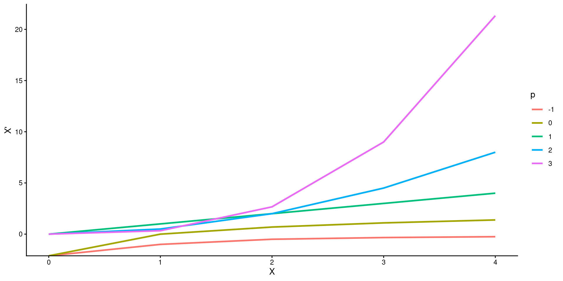
The Box-Cox family of modified power transformations, \(X^{(p)}= (X^p - 1)/p\), for values of \(p = -1, 0, 1, 2, 3\). When \(p = 0, X^{(p)} = log_e X\).
The power transformation \(X^{(0)}\) is useless, but the very useful log transformation is a kind of zero power:
where \(e \approx 2.718\) is the base of the natural logarithms. Thus, we will take \(X^{(0)} \equiv log(X)\).
It is generally more convenient to use logs to the base 10 or base 2, which are more easily interpreted than logs to the base e.
Changing bases is equivalent to multiplying your variable by a constant. No effect on significance tests.
Descending the ladder of powers and roots from \(p = 1\) (i.e., no transformation) towards \(p = -2\)compresses the large values of X and spreads out the small ones.
Ascending the ladder of powers from \(p = 1\) towards \(p = 3\) has the opposite effect.
Power transformations are sensible only when all of the values of \(X\) are positive:
Some of the transformations, such as log (\(p= 0\)) and square root (\(p= .5\)), are undefined for negative or zero values of \(X\).
Power transformations are not monotone (i.e., they change to order of scores) when there are both positive and negative values among the data.
We can add a positive constant (called a start) to each data value to make all of the values positive:
\(X\) → \((X + s)^{(p)}\)
Power transformations are effective only when the ratio of the biggest data values to the smallest ones is sufficiently large; if this ratio is close to 1, then power transformations are nearly linear. For example:
Power transformations will work well if range of \(X = 1 – 100\).
Power transformations will have little effect if range of \(X = 1000 – 1100\)
Using a negative start can often increase the ratio of highest/lowest score.
Using reasonable starts, if necessary, an adequate power transformation can usually be found in the range \(−2 \le p \le 3\).
Power transformations of \(Y\) (or sometimes \(X\)) can correct problems with normality of errors.
Power transformations of \(Y\) (or sometimes \(X\)) can stabilize the variance of the errors.
Power transformations of \(X\) (or sometimes \(Y\)) can make many nonlinear relationships more nearly linear.
You can experiment with Box-Cox transformations of \(X\) or \(Y\) in R using bcPower() in the car package.
In many fields, \(X^p\) rather than \(X^{(p)}\) may be preferred. Particularly, if \(p \ge 0\). This is simply done algebraically.
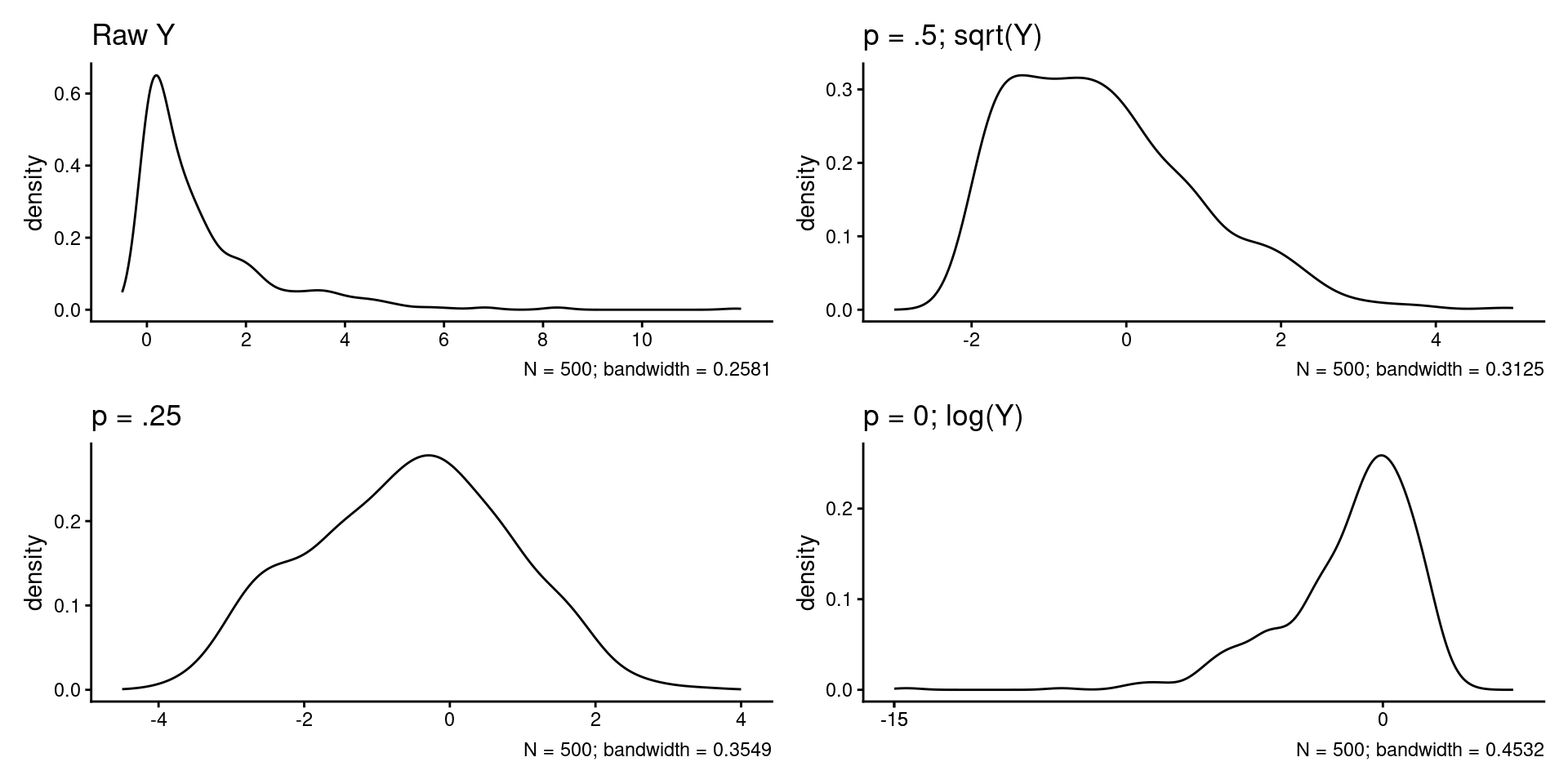
Transformations: Dealing with Skew
Transforming \(Y\)down the ladder can correct positive skew in the errors (most common problem).
Transforming \(Y\)up the ladder corrects negative skew in the errors.
Transforming \(Y\)down the ladder can correct problems with increasing spread of errors as \(Y\) increases (most common problem).
Transforming \(Y\)up the ladder corrects decreasing spread.
The problems of unequal spread and skewness commonly occur together and can be corrected together. Therefore, transforming \(Y\) down the ladder can correct both issues simultaneously.
Lets return to the FPS example from the previous units and fit the 3 predictor model
path_data <-"data_lecture"data <-read_csv(here::here(path_data, "09_transformations_fps.csv"), show_col_types =FALSE) |>mutate(sex_c =if_else(sex =="female", -.5, .5)) |># remove outliers to fit same model as last two units filter(!subid %in%c("0125", "2112"))m <-lm(fps ~ bac + ta + sex_c, data = data)summary(m)
Call:
lm(formula = fps ~ bac + ta + sex_c, data = data)

Residuals:
    Min      1Q  Median      3Q     Max
-63.419 -15.870  -3.955  14.992  81.050

Coefficients:
              Estimate Std. Error t value  Pr(>|t|)
(Intercept)   28.70270    6.44222   4.455 0.0000240 ***
bac         -254.58936   72.18588  -3.527  0.000664 ***
ta             0.12306    0.02726   4.514 0.0000192 ***
sex_c        -15.85499    5.69071  -2.786  0.006505 **
---
Signif. codes:  0 '***' 0.001 '**' 0.01 '*' 0.05 '.' 0.1 ' ' 1

Residual standard error: 27.49 on 90 degrees of freedom
Multiple R-squared:  0.3191,    Adjusted R-squared:  0.2964
F-statistic: 14.06 on 3 and 90 DF,  p-value: 0.0000001355
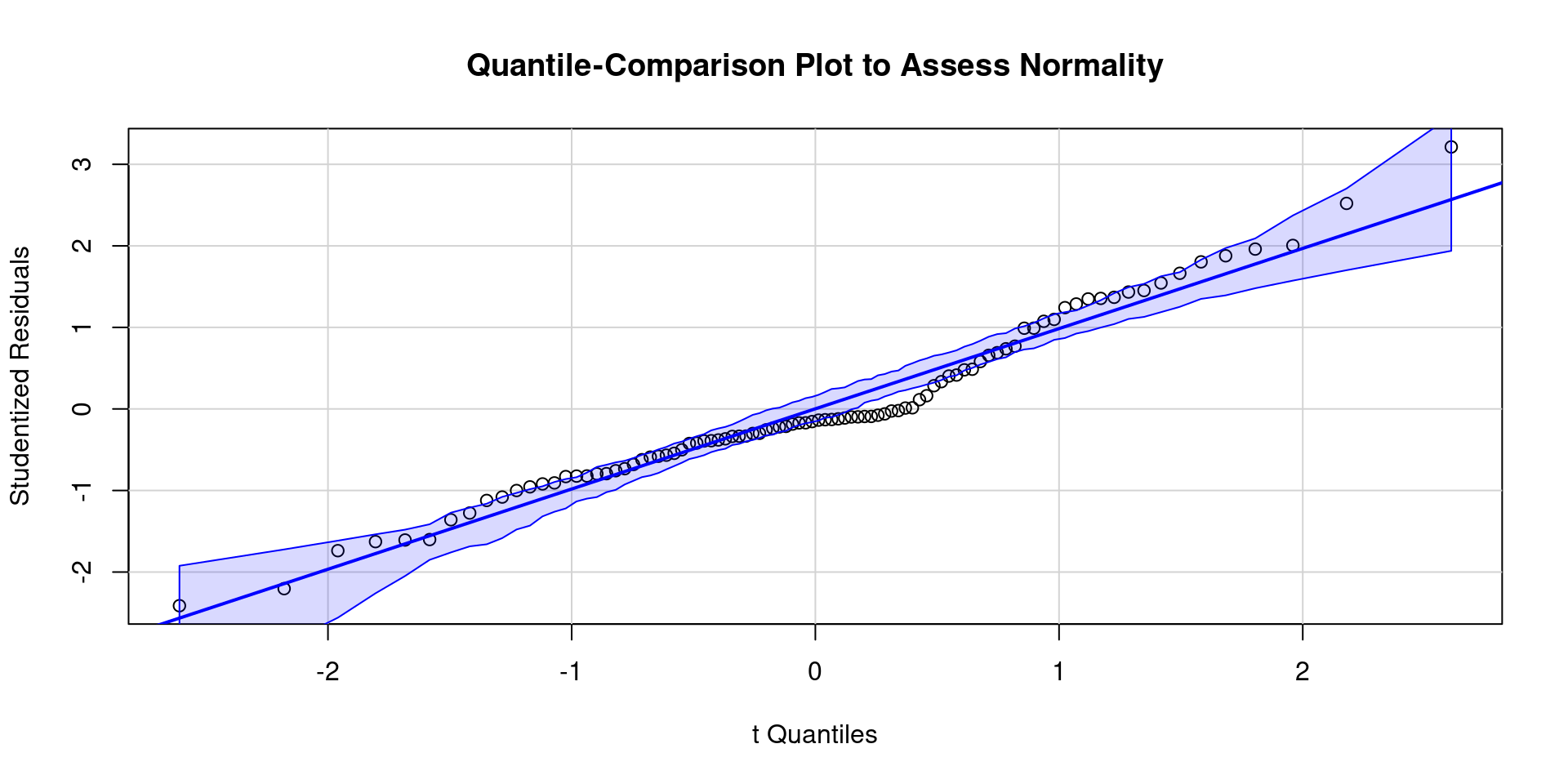
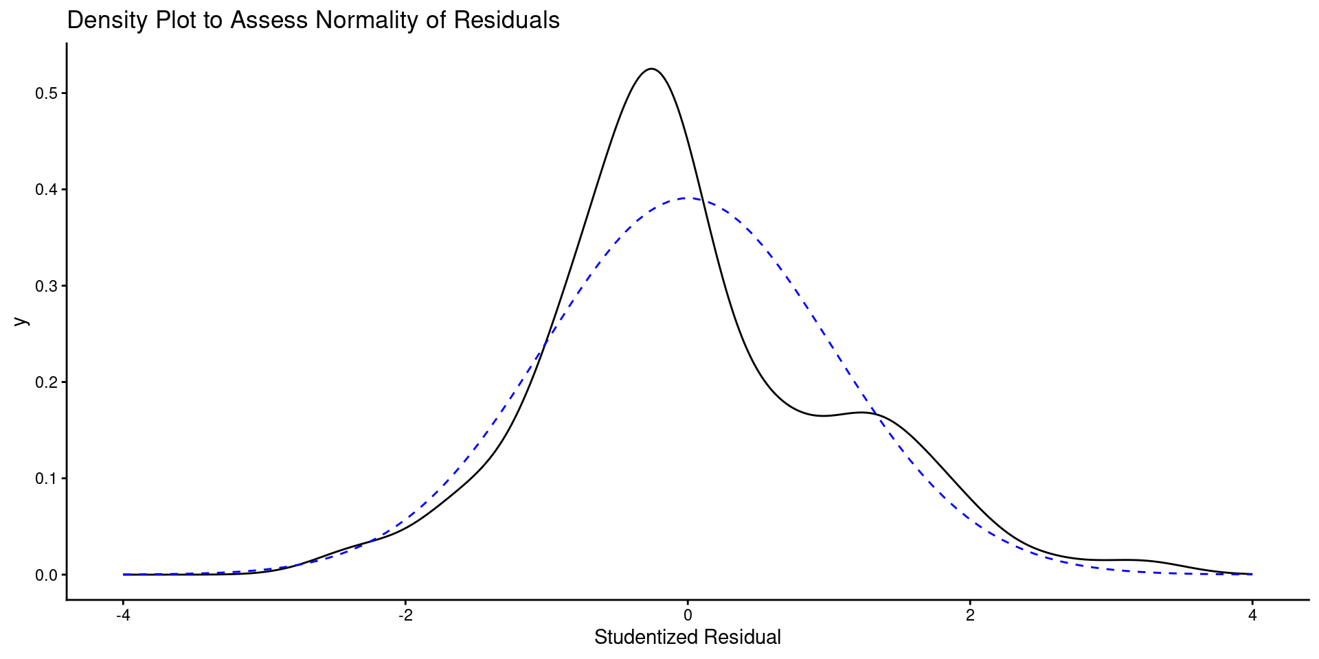
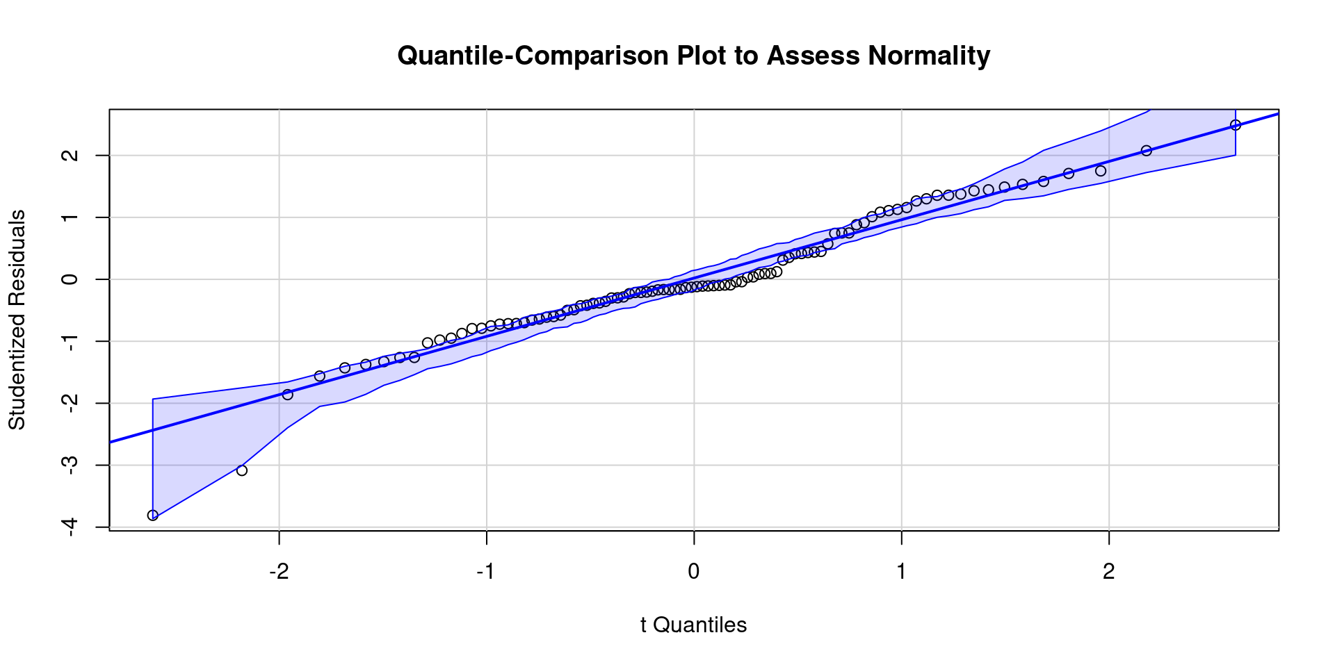
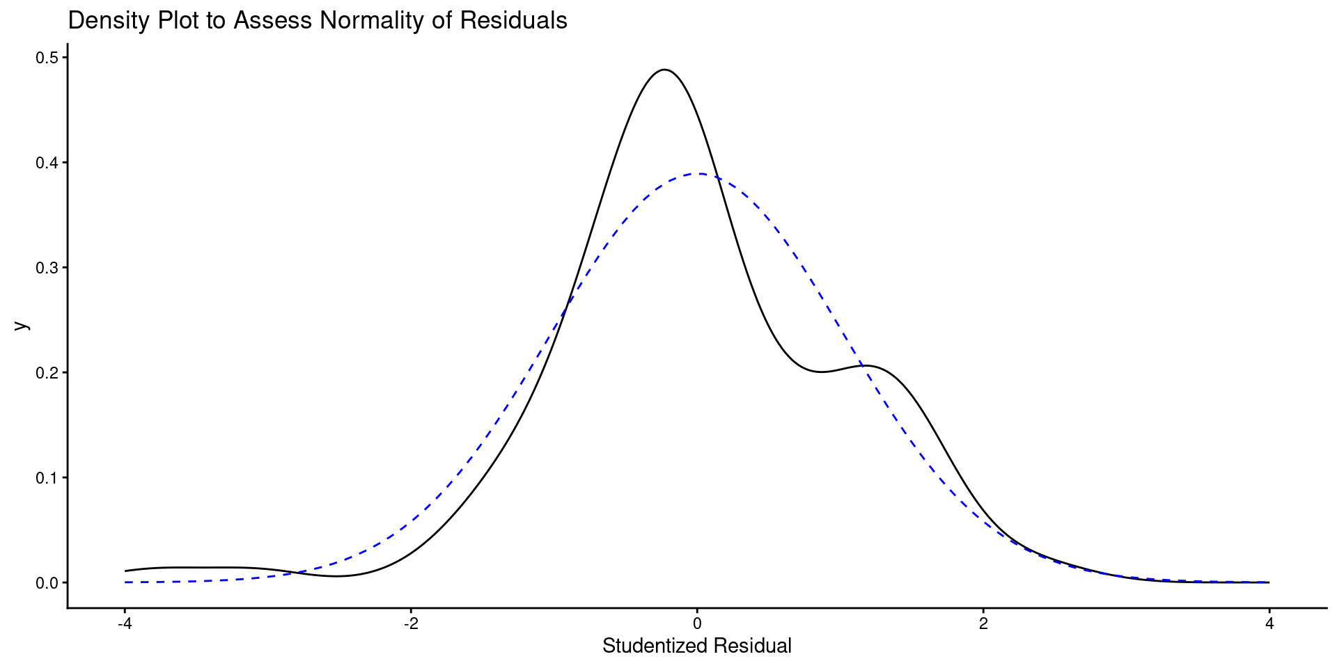
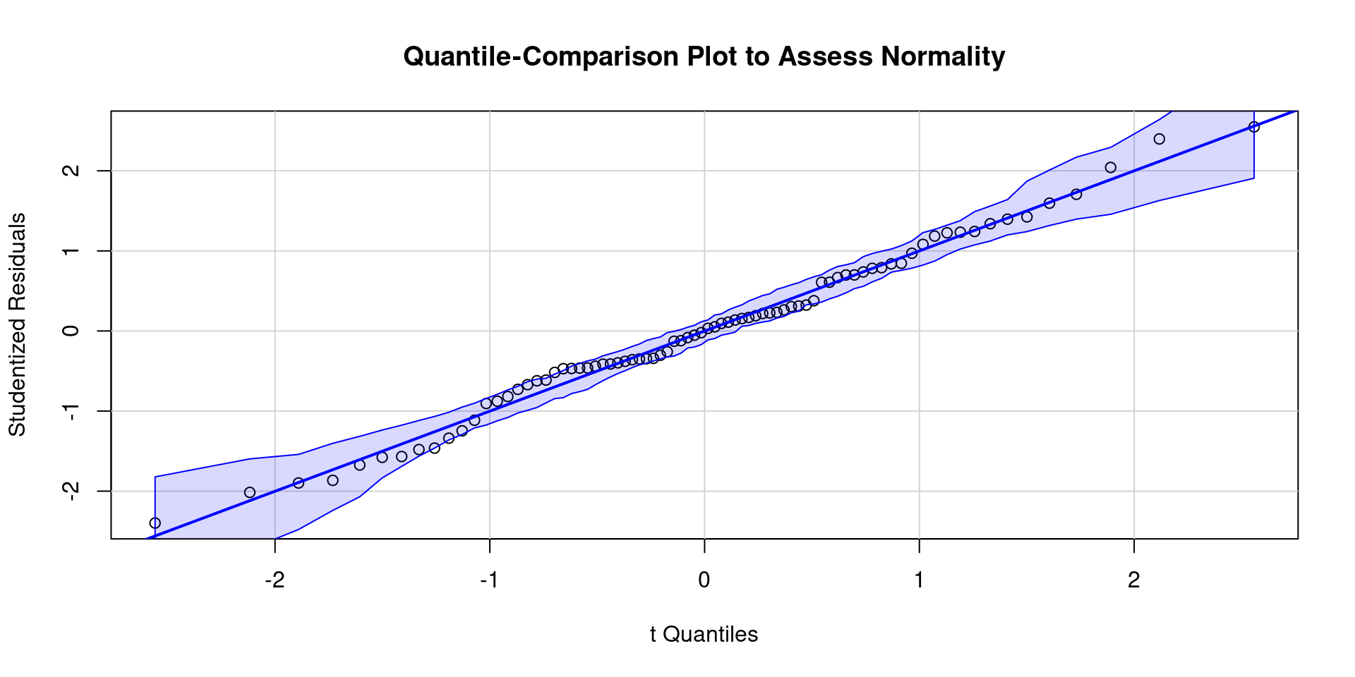
Let review model assumptions
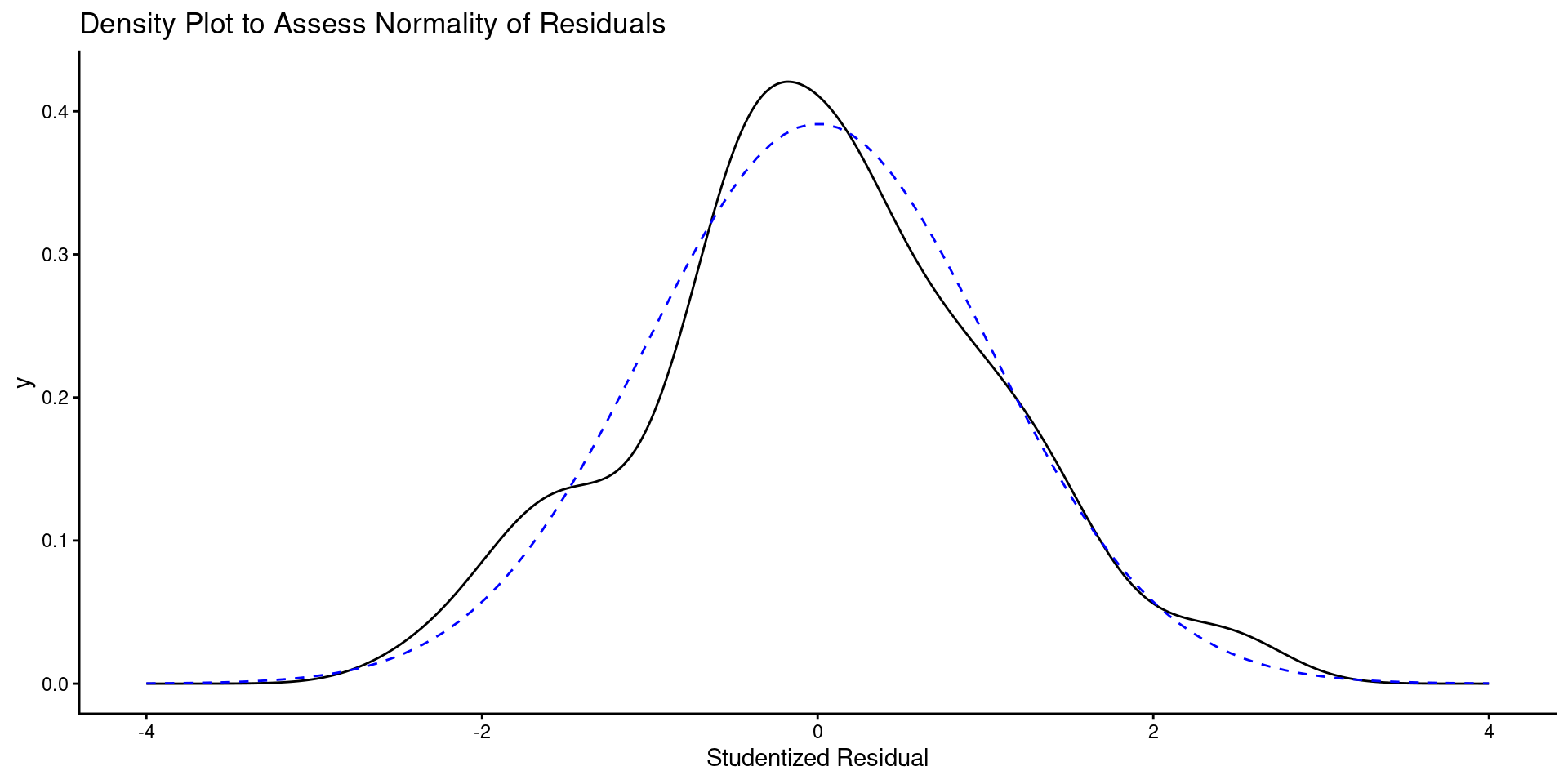
Here is a QQ plot and a density plot of residuals
Code
car::qqPlot(m, id =FALSE, simulate =TRUE,main ="Quantile-Comparison Plot to Assess Normality", ylab ="Studentized Residuals")
Code
ggplot() +geom_density(aes(x = value), data =enframe(rstudent(m), name =NULL)) +labs(title ="Density Plot to Assess Normality of Residuals",x ="Studentized Residual") +geom_line(aes(x = x, y = y), data =tibble(x =seq(-4, 4, length.out =100),y =dnorm(seq(-4, 4, length.out =100), mean=0, sd=sd(rstudent(m)))), linetype ="dashed", color ="blue")
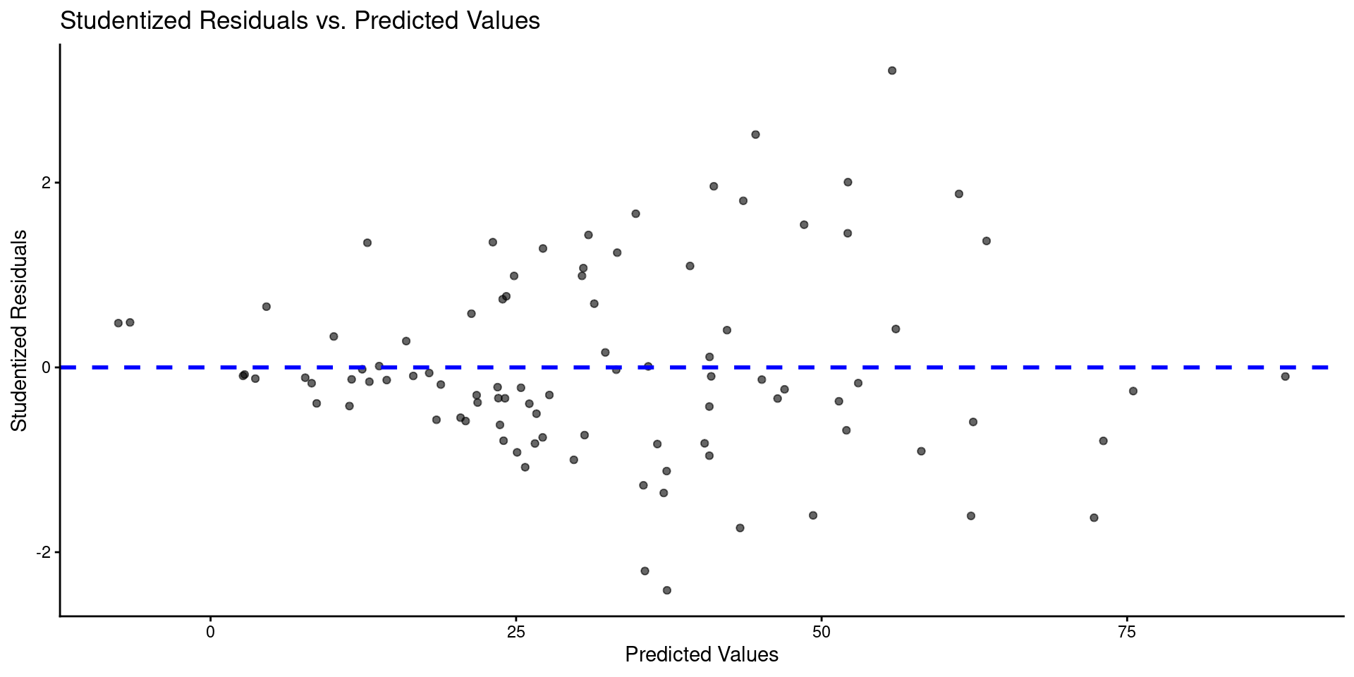
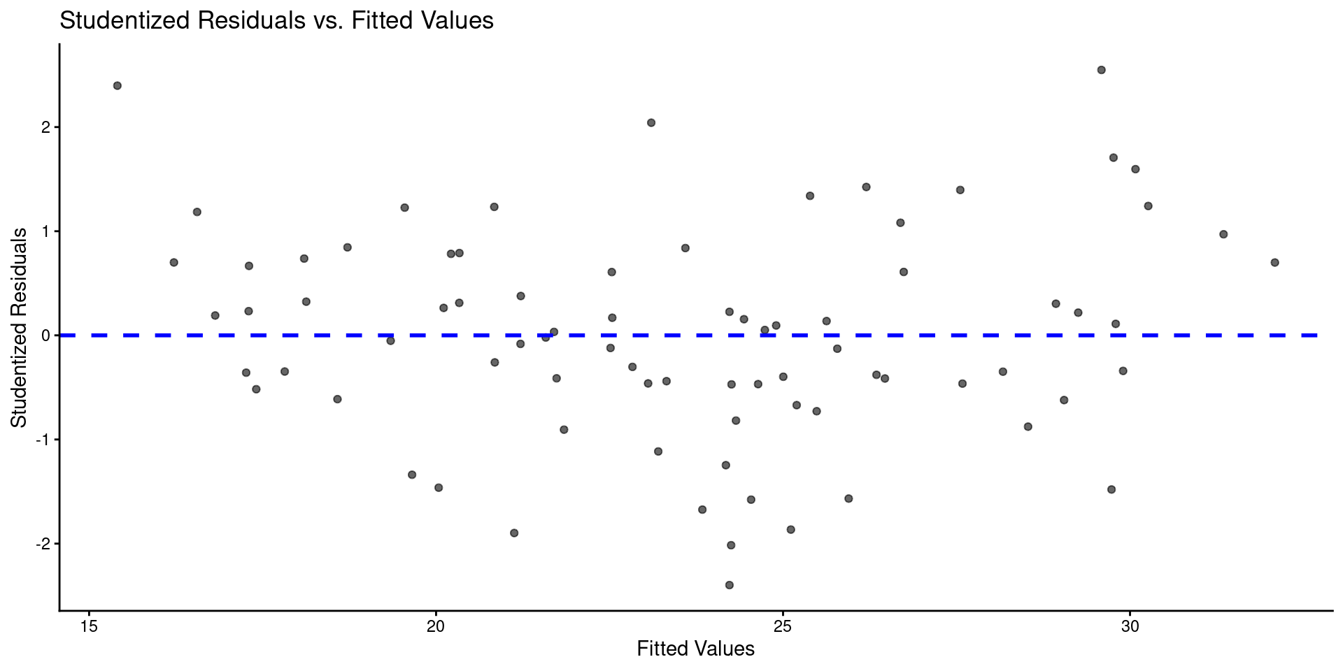
Here is a plot of residuals by predicted values
tibble(y_hat =predict(m),res =rstudent(m)) |>ggplot(aes(x = y_hat, y = res)) +geom_point(alpha = .6) +geom_hline(yintercept =0, linetype ="dashed", color ="blue", linewidth =1) +labs(title ="Studentized Residuals vs. Predicted Values",x ="Predicted Values",y ="Studentized Residuals")
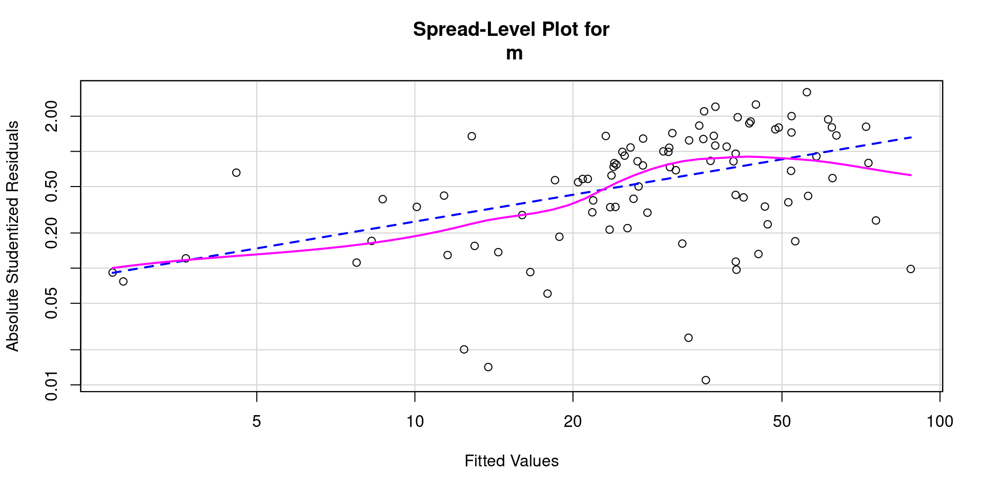
And a spread level plot
m |> car::spreadLevelPlot()
Suggested power transformation: 0.2370356
And statistical test for non-constant variance
m |> car::ncvTest()
Non-constant Variance Score Test
Variance formula: ~ fitted.values
Chisquare = 13.2232, Df = 1, p = 0.00027651
And global tests of model assumptions
m |> gvlma::gvlma()
Call:
lm(formula = fps ~ bac + ta + sex_c, data = data)

Coefficients:
(Intercept)          bac           ta        sex_c
    28.7027    -254.5894       0.1231     -15.8550


ASSESSMENT OF THE LINEAR MODEL ASSUMPTIONS
USING THE GLOBAL TEST ON 4 DEGREES-OF-FREEDOM:
Level of Significance =  0.05

Call:
 gvlma::gvlma(x = m)

                        Value p-value                   Decision
Global Stat        9.39689053 0.05191    Assumptions acceptable.
Skewness           3.60145982 0.05773    Assumptions acceptable.
Kurtosis           0.30834234 0.57870    Assumptions acceptable.
Link Function      0.00002503 0.99601    Assumptions acceptable.
Heteroscedasticity 5.48706334 0.01916 Assumptions NOT satisfied!
Box Cox Transformation Function
data |>select(bac, ta, sex_c, fps) |>skim() |>focus(n_missing, numeric.mean, numeric.sd, min = numeric.p0, max = numeric.p100) |>yank("numeric")
Variable type: numeric
skim_variable
n_missing
mean
sd
min
max
bac
0
0.06
0.04
0.00
0.14
ta
0
145.91
104.80
10.00
445.00
sex_c
0
0.01
0.50
-0.50
0.50
fps
0
32.19
32.77
-26.07
136.82
We are going to first add a constant so all response values are > 0
data <- data |>mutate(fps_27 = fps +27)m_2 <-lm(fps_27 ~ bac + ta + sex_c, data = data)
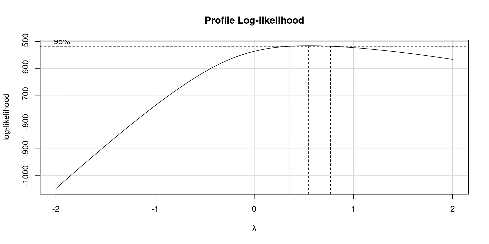
Next we will pull the best lambda value from a plot of log-likelihood values by lambda power transformations of response variable.
Lastly, we will use the best lambda value to conduct our power transformation and re-evaluate our model assumptions.
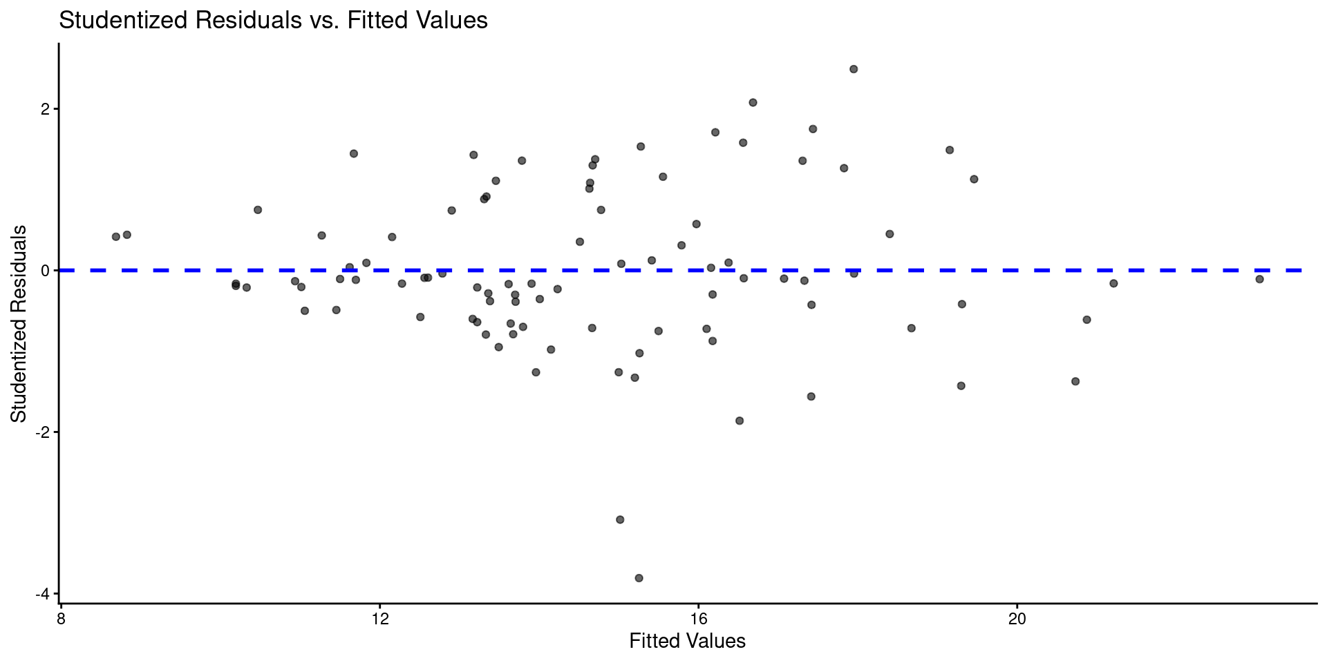
data <- data |>mutate(fps_bc = car::bcPower(fps_27, .55))m_3 <-lm(fps_bc ~ bac + ta + sex_c, data = data)
Code
car::qqPlot(m_3, id =FALSE, simulate =TRUE, main ="Quantile-Comparison Plot to Assess Normality", ylab ="Studentized Residuals")
Code
ggplot() +geom_density(aes(x = value), data =enframe(rstudent(m_3), name =NULL)) +labs(title ="Density Plot to Assess Normality of Residuals",x ="Studentized Residual") +geom_line(aes(x = x, y = y), data =tibble(x =seq(-4, 4, length.out =100),y =dnorm(seq(-4, 4, length.out =100), mean=0, sd=sd(rstudent(m_3)))), linetype ="dashed", color ="blue")
Code
tibble(x =fitted.values(m_3),y =rstudent(m_3)) |>ggplot(aes(x = x, y = y)) +geom_point(alpha = .6) +geom_hline(yintercept =0, linetype ="dashed", color ="blue", linewidth =1) +labs(title ="Studentized Residuals vs. Fitted Values",x ="Fitted Values",y ="Studentized Residuals")
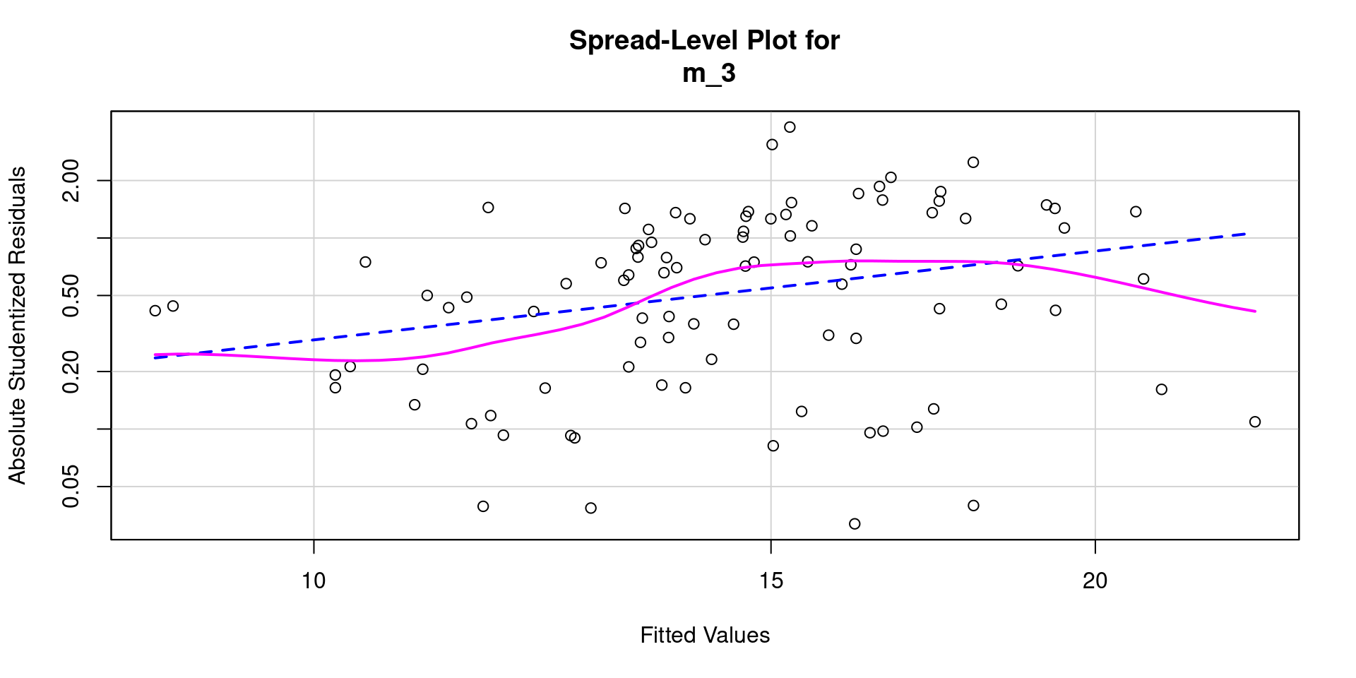
car::spreadLevelPlot(m_3)
Suggested power transformation: -0.5446104
Code
car::ncvTest(m_3)
Non-constant Variance Score Test
Variance formula: ~ fitted.values
Chisquare = 6.005664, Df = 1, p = 0.01426
Code
gvlma::gvlma(m_3)
Call:
lm(formula = fps_bc ~ bac + ta + sex_c, data = data)

Coefficients:
(Intercept)          bac           ta        sex_c
   14.21548    -37.52098      0.01793     -2.70290


ASSESSMENT OF THE LINEAR MODEL ASSUMPTIONS
USING THE GLOBAL TEST ON 4 DEGREES-OF-FREEDOM:
Level of Significance =  0.05

Call:
 gvlma::gvlma(x = m_3)

                       Value p-value                   Decision
Global Stat        12.759981 0.01251 Assumptions NOT satisfied!
Skewness            1.588199 0.20758    Assumptions acceptable.
Kurtosis            5.520612 0.01879 Assumptions NOT satisfied!
Link Function       0.004907 0.94416    Assumptions acceptable.
Heteroscedasticity  5.646263 0.01749 Assumptions NOT satisfied!
Maybe better choicer was untransformed Y (original model) with corrected SEs?
Maybe the problem wasn’t bad enough to do anything?
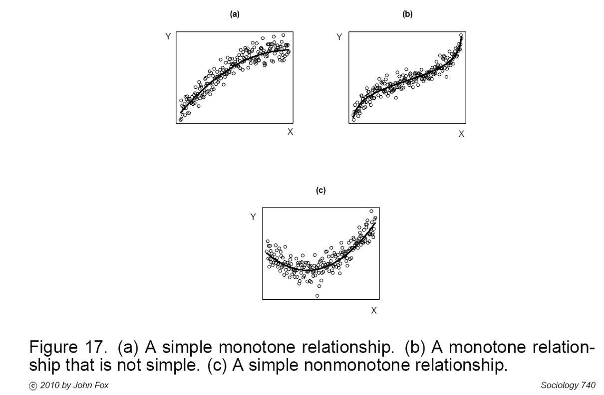
Transformations: Dealing with Non-linearity
Power transformations can make simple monotone relationships more linear (Fig A). Polynomial regression (or other transformations, e.g. logit) is often needed for more complex relationships (Figs, B & C).
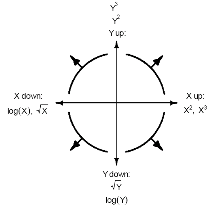
Transformations: Mosteller and Tukey’s bulging rule
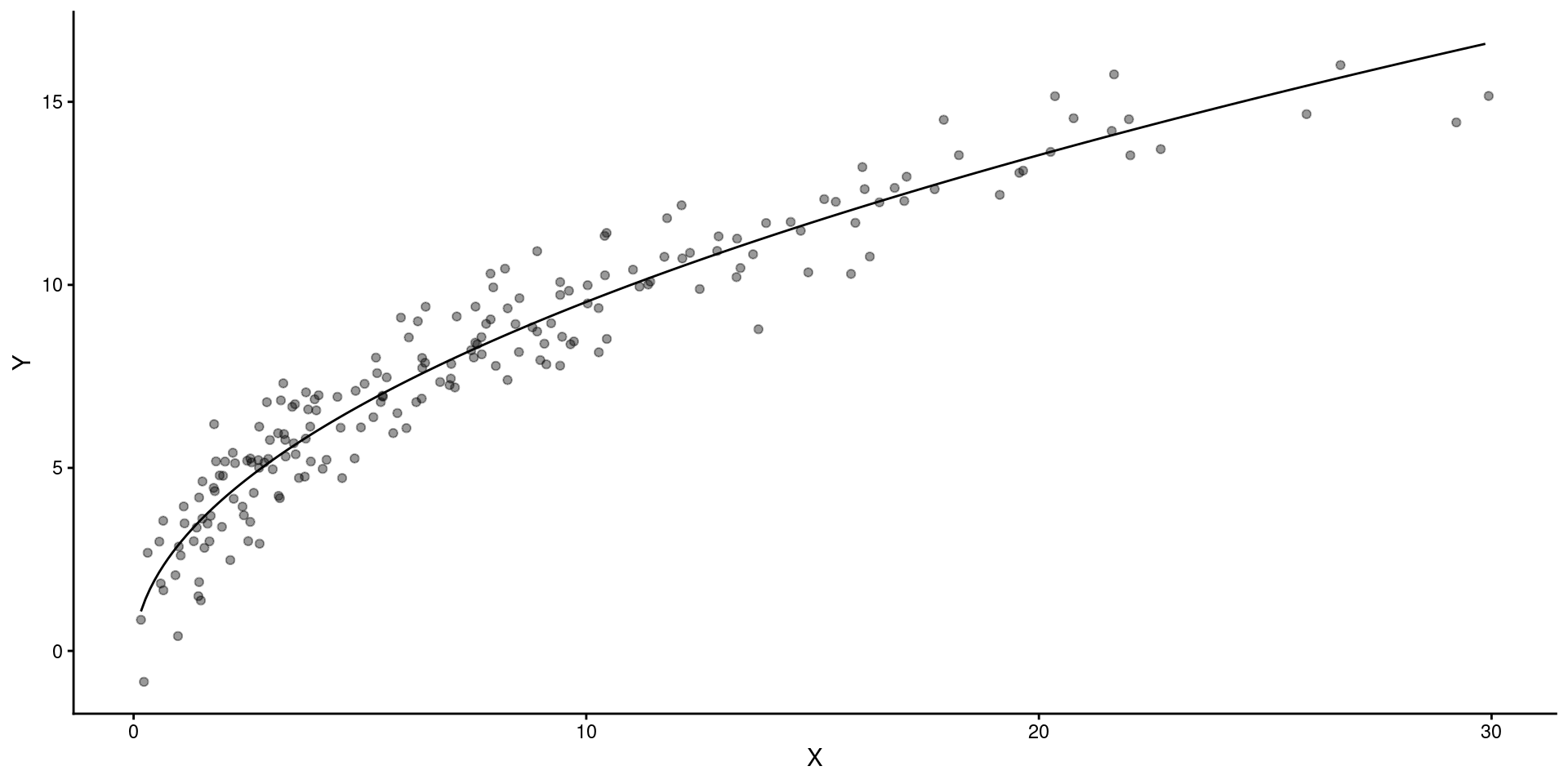
Simple monotone relationships can be corrected by transforming \(X\) or \(Y\).
\(X\) is typical if only one \(XY\) relationship is problematic.
If all \(X\)s have similar non-linear relationship, transform \(Y\).
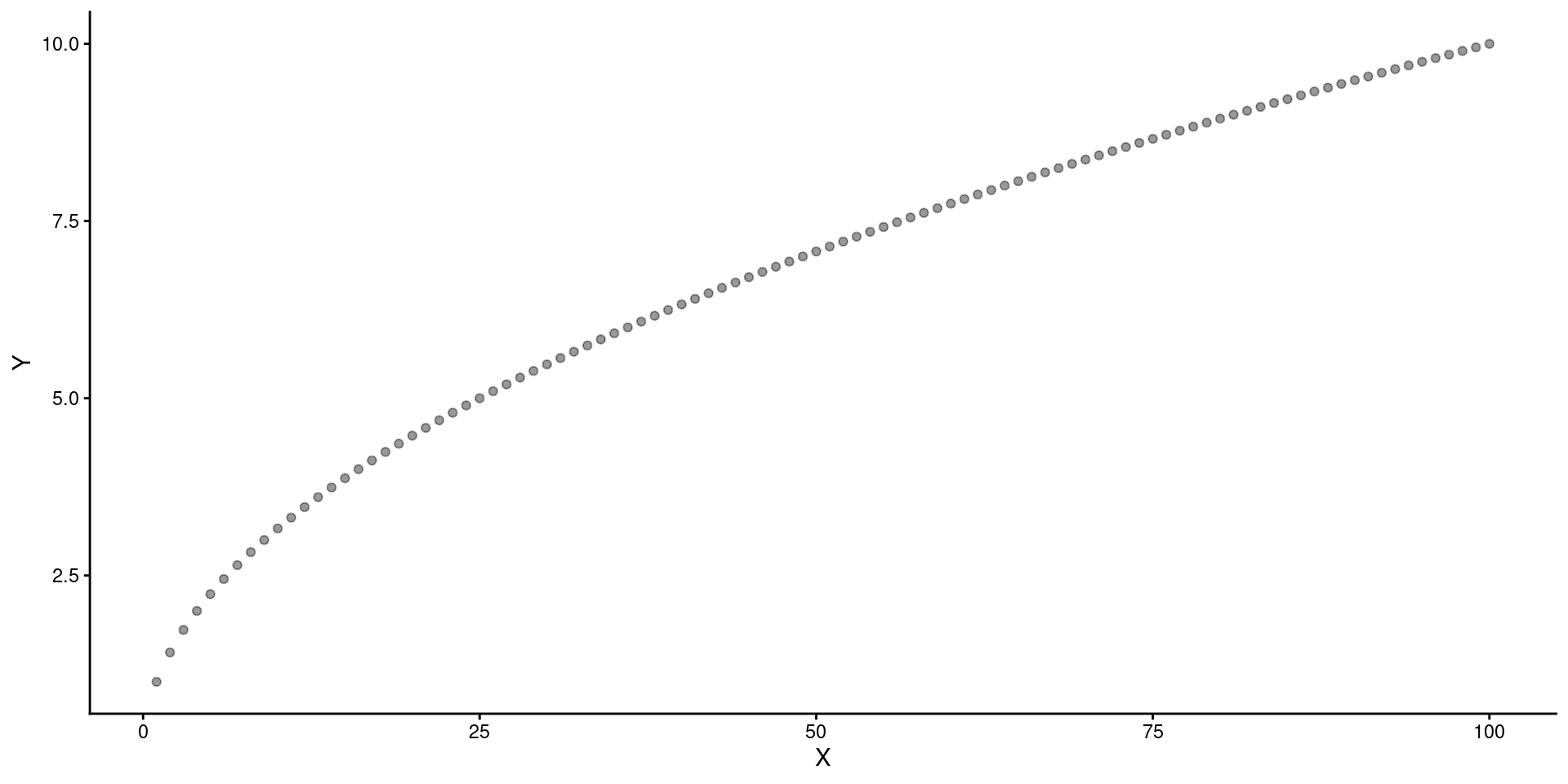
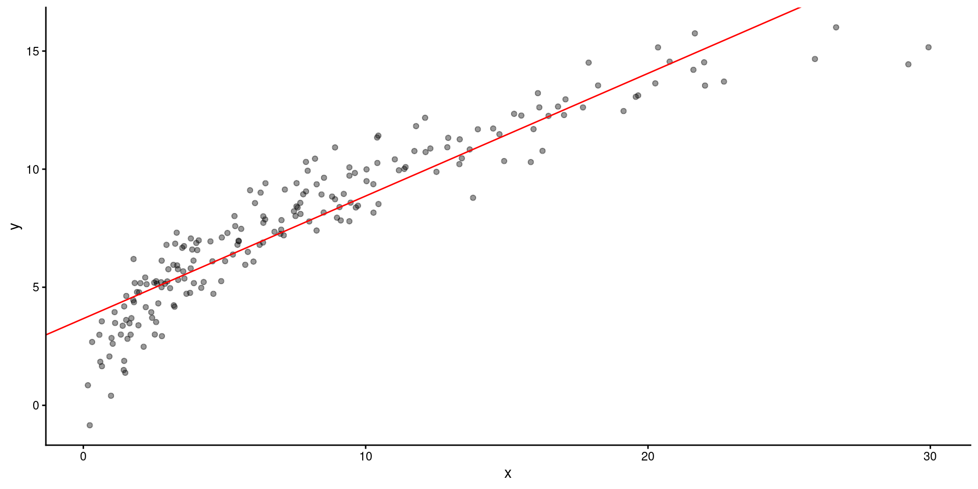
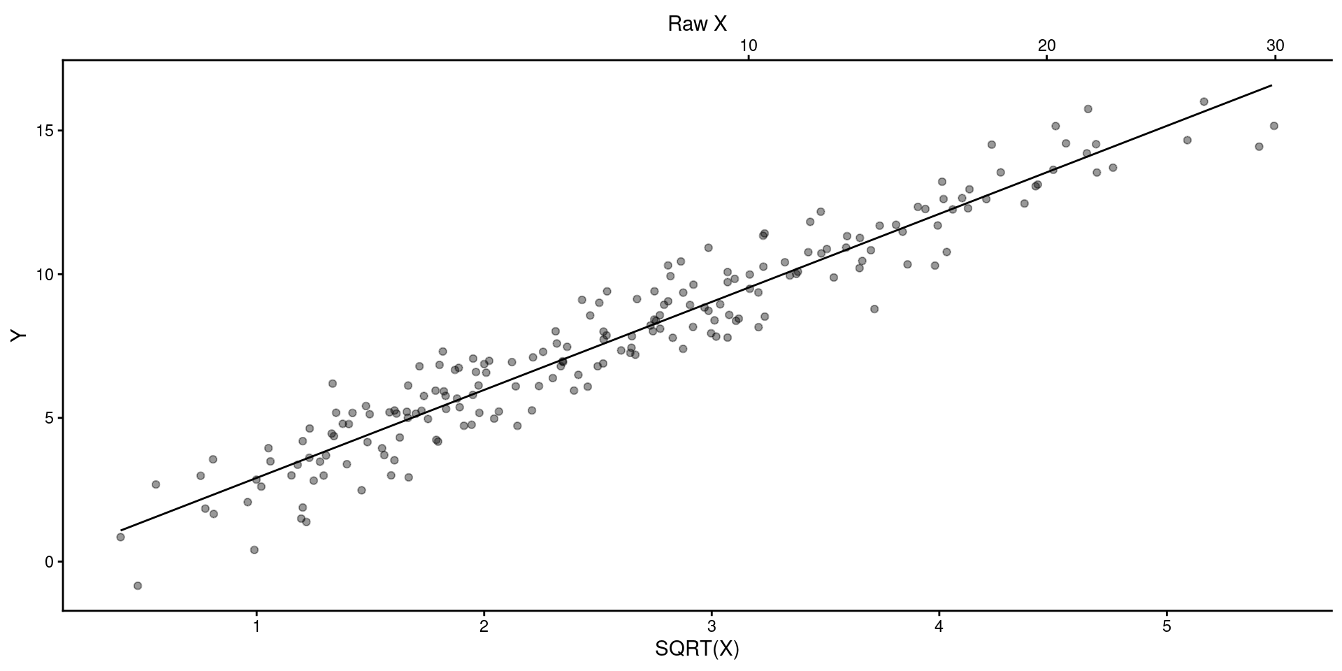
Question
What 2 transformations would make this relationship linear?
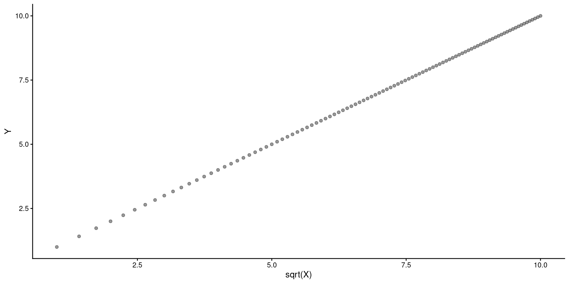
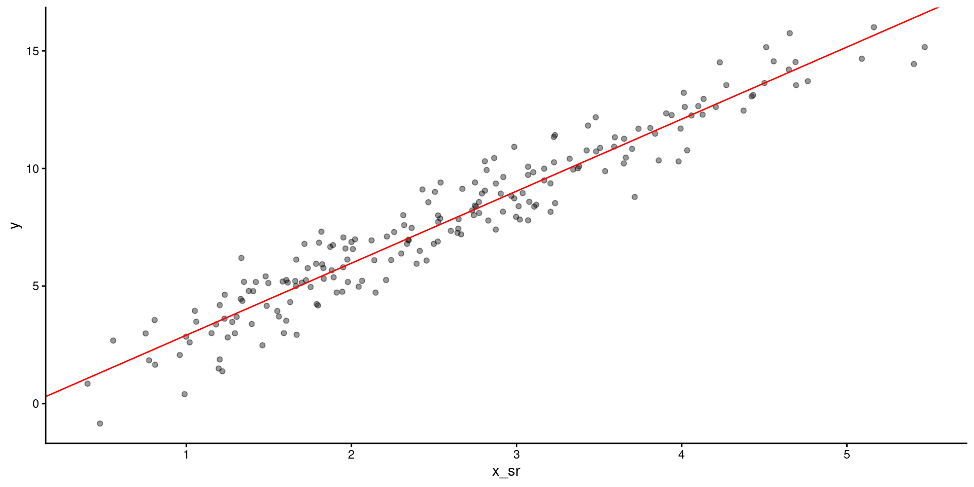
Move \(X\) down the ladder (e.g., \(X^.5\)).
data_nonlinear |>ggplot(aes(x =sqrt(X), y = Y)) +geom_point(alpha = .4)
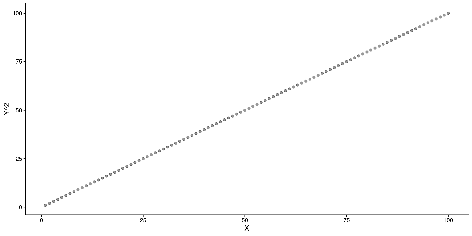
Move \(Y\) up the ladder (e.g., \(Y^2\)).
data_nonlinear |>ggplot(aes(x = X, y = Y^2)) +geom_point(alpha = .4)
General Transformations
In some fields, certain power transformations (sqrt, log, inverse) are common.
If we have a choice between transformations that perform roughly equally well, we may prefer one transformation to another because of interpretability:
The log transformation has a convenient multiplicative interpretation (e.g., increasing log2 (X) by 1 doubles X; increasing log10 (X) by 1 multiples X by 10).
Transformations are a big source of research dfs. Should be pre-registered. You may know what your DV typically needs from prior data. Worst case, report with and without transformations and justify.
m_5k <-lm(time ~ age + miles, data = data_5k)broom::tidy(m_5k)
# A tibble: 3 × 5
  term        estimate std.error statistic  p.value
  <chr>          <dbl>     <dbl>     <dbl>    <dbl>
1 (Intercept)   25.0      1.80       13.9  1.07e-22
2 age            0.172    0.0333      5.17 1.77e- 6
3 miles         -0.210    0.0246     -8.53 9.54e-13
Code
car::qqPlot(m_5k, id =FALSE, simulate =TRUE,main ="Quantile-Comparison Plot to Assess Normality", ylab ="Studentized Residuals")
Code
ggplot() +geom_density(aes(x = value), data =enframe(rstudent(m_5k), name =NULL)) +labs(title ="Density Plot to Assess Normality of Residuals",x ="Studentized Residual") +geom_line(aes(x = x, y = y), data =tibble(x =seq(-4, 4, length.out =100),y =dnorm(seq(-4, 4, length.out =100), mean=0, sd=sd(rstudent(m_5k)))), linetype ="dashed", color ="blue")
Code
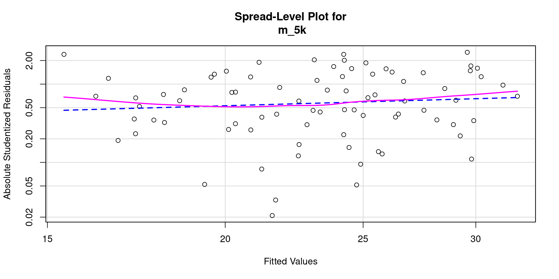
tibble(x =fitted.values(m_5k),y =rstudent(m_5k)) |>ggplot(aes(x = x, y = y)) +geom_point(alpha = .6) +geom_hline(yintercept =0, linetype ="dashed", color ="blue", linewidth =1) +labs(title ="Studentized Residuals vs. Fitted Values",x ="Fitted Values",y ="Studentized Residuals")
car::spreadLevelPlot(m_5k)
Suggested power transformation: 0.4894249
car::ncvTest(m_5k)
Non-constant Variance Score Test
Variance formula: ~ fitted.values
Chisquare = 0.8077899, Df = 1, p = 0.36877
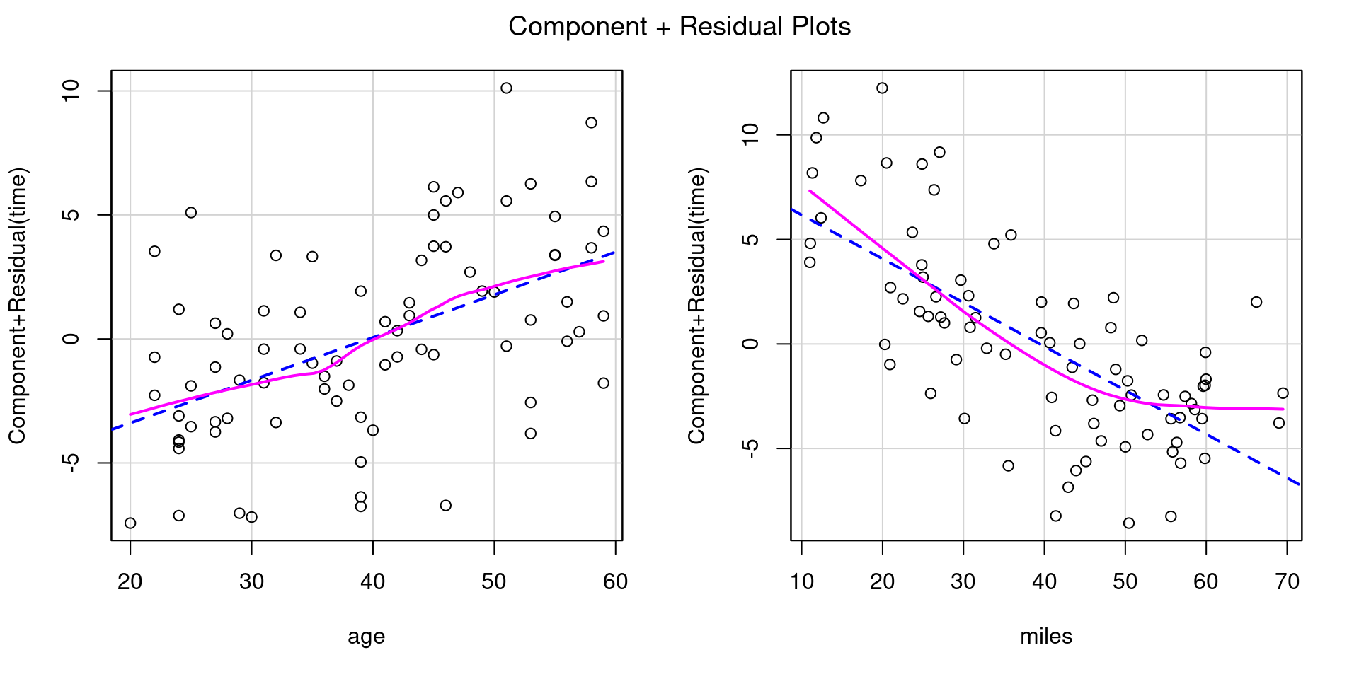
car::crPlots(m_5k, ask =FALSE)
gvlma::gvlma(m_5k)
Call:
lm(formula = time ~ age + miles, data = data_5k)

Coefficients:
(Intercept)          age        miles
    24.9804       0.1724      -0.2097


ASSESSMENT OF THE LINEAR MODEL ASSUMPTIONS
USING THE GLOBAL TEST ON 4 DEGREES-OF-FREEDOM:
Level of Significance =  0.05

Call:
 gvlma::gvlma(x = m_5k)

                      Value   p-value                   Decision
Global Stat        13.01039 0.0112252 Assumptions NOT satisfied!
Skewness            0.01435 0.9046389    Assumptions acceptable.
Kurtosis            0.07603 0.7827462    Assumptions acceptable.
Link Function      12.82570 0.0003419 Assumptions NOT satisfied!
Heteroscedasticity  0.09430 0.7587759    Assumptions acceptable.
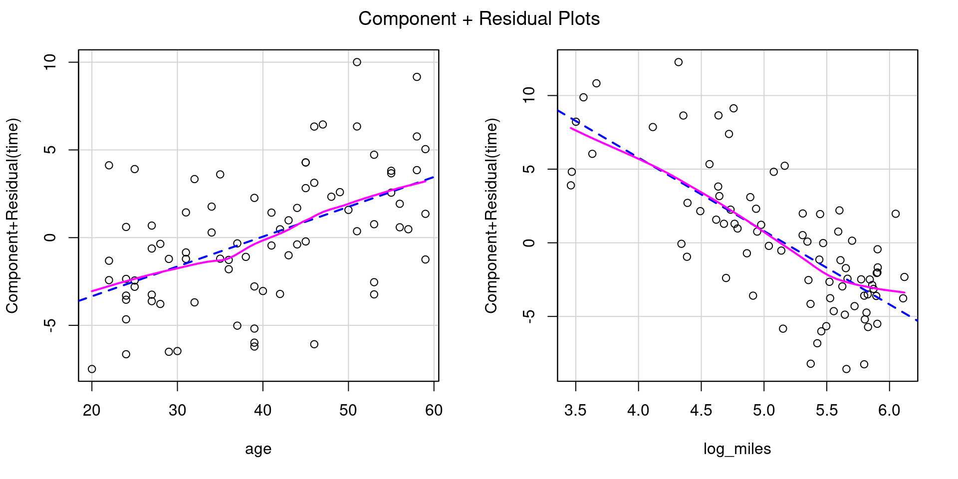
Let’s try transforming miles using log2(), a binary logarithm (base 2).
data_5k <- data_5k |>mutate(log_miles =log2(miles))m_5k_tran <-lm(time ~ age + log_miles, data = data_5k)broom::tidy(m_5k_tran)
Call:
lm(formula = time ~ age + log_miles, data = data_5k)

Coefficients:
(Intercept)          age    log_miles
     42.519        0.170       -4.983


ASSESSMENT OF THE LINEAR MODEL ASSUMPTIONS
USING THE GLOBAL TEST ON 4 DEGREES-OF-FREEDOM:
Level of Significance =  0.05

Call:
 gvlma::gvlma(x = m_5k_tran)

                     Value p-value                Decision
Global Stat        1.83180  0.7667 Assumptions acceptable.
Skewness           0.15584  0.6930 Assumptions acceptable.
Kurtosis           0.06402  0.8003 Assumptions acceptable.
Link Function      1.58986  0.2073 Assumptions acceptable.
Heteroscedasticity 0.02209  0.8819 Assumptions acceptable.